Go schemaless: ELT with Google Cloud Storage and BigQuery

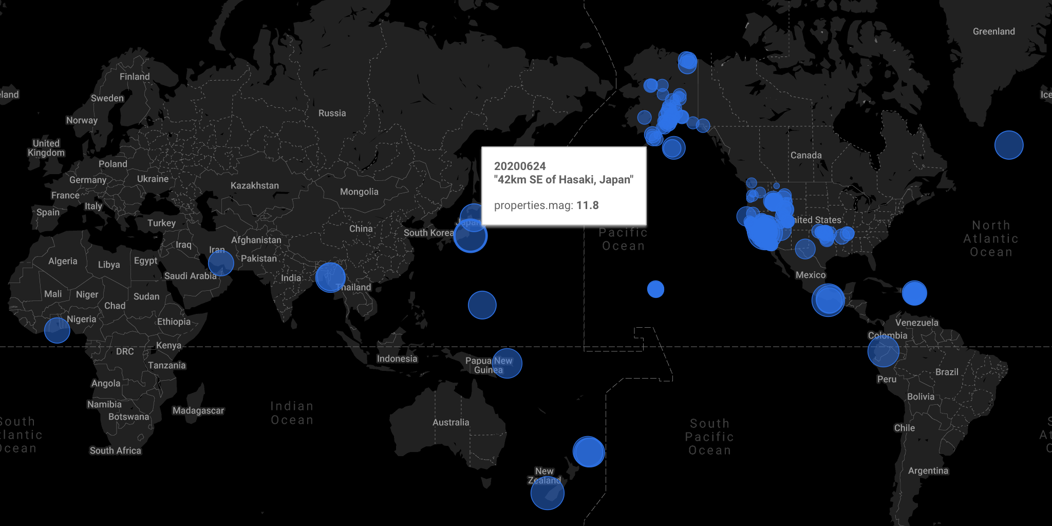
The image above, generated with the data in this article,
is a map showing the location and magnitude (bubble size) of earthquakes on June 24, 2020, based on the USGS Earthquake event data.

Load first. Worry about schema later.

When we load the data to a data warehouse, we usually
specify the schema
upfront.
What if we can first load the data without worrying about the schema,
and format the data on the data warehouse?

In a typical ETL (Extract, Transform, and Load) framework, the data is

1. Extracted from the source.
2. Transformed. The transformation includes formatting to a pre-defined schema.
3. Loaded to a data store such as a data warehouse.

The advantages of doing ELT (Extract, Load, and Transform) instead of include:

1. The extraction process won’t have to change when the schema changes.
2. The transformation process can take advantage of the massively-parallel execution by the modern data warehouse.

In this post, I would like to demonstrate the business impact, especially with speed, when we adopt ELT approach.

ELT with BigQuery and Cloud Storage

In Google Cloud Platform, it is very easy to do ELT with
Cloud Storage
and BigQuery. Using GCS and BigQuery, Felipe Hoffa demonstrated a lazy-loading of half a trillion Wikipedia page views.
(His articles can be found here and here)

In his post, Hoffa loaded the super large set of files with a simple format (space-separated) parsing with REGEXP_EXTRACT function.
I will use
the USGS Earthquake event data as an example dataset. The earthquake event data is a newline-separated JSON file that looks like this:

{
  "type":"Feature",
  "properties":{
    "mag":1.1000000000000001,
    "place":"117km NW of Talkeetna, Alaska",
    "time":1388620046501,
    "updated":1558392330681,
    "tz":-540,
    ...
    "type":"earthquake",
    "title":"M 1.1 - 117km NW of Talkeetna, Alaska"
  },
  "geometry":{
    "type":"Point",
    "coordinates":[
      -151.64590000000001,
      63.101999999999997,
      14.1
    ]
  },
  "id":"ak01421ig3u"
},
{
  "type":"Feature",
  "properties":{
    "mag":1.2,
    "place":"6km SSW of Big Lake, Alaska",
    "time":1388619956476,
    "updated":1558392330249,
    "tz":-540,
    ...

    "type":"earthquake",
    "title":"M 1.2 - 6km SSW of Big Lake, Alaska"
  },
  "geometry":{
    "type":"Point",
    "coordinates":[
      -150.01650000000001,
      61.458100000000002,
      44.600000000000001
    ]
  },
  "id":"ak01421i2zj"
},

stdin to GCS

I wrote target_gcs,
a Python program that takes stdin and writes out to a Cloud Storage location. It is easy to install via pip:

python3 -m venv ./venv
source ./venv/bin/activate
pip install https://github.com/anelendata/target_gcs/tarball/master

Then follow the instruction to configure the Google Cloud Platform project and data location.

After the simple set up, you can run

curl "https://earthquake.usgs.gov/fdsnws/event/1/query?format=geojson&starttime=2020-06-24&endtime=2020-06-25" | \
target_gcs -c ./your-config.json

to get the data loaded on Cloud Storage.
In this simple example, the USGS data is fetched by curl command,
and the data is written out to stdout.
target_gcs receives the data through pipe (|) and writes out to GCS.

GCS to BigQuery

After the data is loaded to Cloud Storage, it’s time to create a table on BigQuery.
For this, we can create an externally partitioned table
with the Python script I provided (*):

python create_schemaless_table.py \
  -p your-project-id \
  -g gs://your-bucket/your-dataset \
  -d your-dataset-name \
  -t your-table-name

In my case, I set the target dataset name to gcs_partitioned
and table name to usgs_events_unparsed.

(*) Note: If the JSON schema in the data is stable and consistent, it makes more sense to load in
the standard way of loading JSON data.
In the method in this article is advantageous when you have JSON record whose set of keys are inconsistent among records.
I also had a case where I needed to first search for all the keys present in the data, then flatten/unwrap/unpivot the data into a long format.

Unstructured data on BigQuery

Let’s query the unstructured data.

SELECT *
FROM `gcs_partitioned.usgs_events_unparsed`
WHERE date BETWEEN DATE '2020-06-24' AND DATE '2020-06-25' LIMIT 10

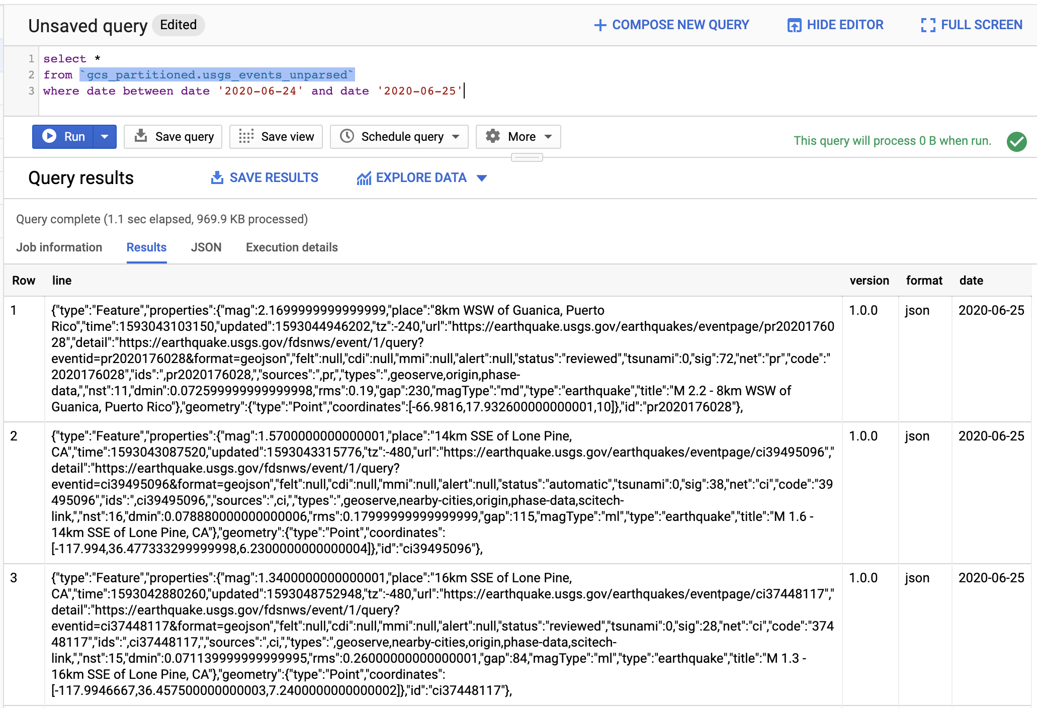
You can see line as the raw JSON string. You also see columns such as version, format, and date.
They are from the GCS file partition information. By using those keys, we can limit the total data scanned with a query.
In fact, the Python script we used to create the BigQuery table from GCS set the option to always require the partition filter in the query.
This is a good practice to avoid running a costly query by accident. (BigQuery costs $5 per TB data scanned.)

Extract the fields from JSON to create a structured view

We can create a view that has the structure from the unstructured table:

CREATE VIEW `views.usgs_events` AS (
  SELECT
    STRUCT(
      TIMESTAMP_MILLIS(
         CAST(JSON_EXTRACT(line,
          '$.properties.time') AS INT64)) AS time,
      CAST(JSON_EXTRACT(line,
          '$.properties.tz') AS INT64) AS tz,
      CAST(JSON_EXTRACT(line,
          '$.properties.mag') AS FLOAT64) AS mag,
      TRIM(JSON_EXTRACT(line,
          '$.properties.place')) AS place ) AS properties,
      CONCAT(JSON_EXTRACT_ARRAY(line, '$.geometry.coordinates')[OFFSET(1)], ',',
             JSON_EXTRACT_ARRAY(line, '$.geometry.coordinates')[OFFSET(0)]) AS lat_lng,
    date AS etl_date
  FROM `gcs_partitioned.usgs_events_unparsed`
  WHERE JSON_EXTRACT(line, '$.type') = '"Feature"'
  )

Here, I’m using functions such as JSON_EXTRACT and JSON_EXTRACT_ARRAY to extract the values from the nested field to create the flat table.
I’m using CAST function to convert the extracted string into the appropriate data types:

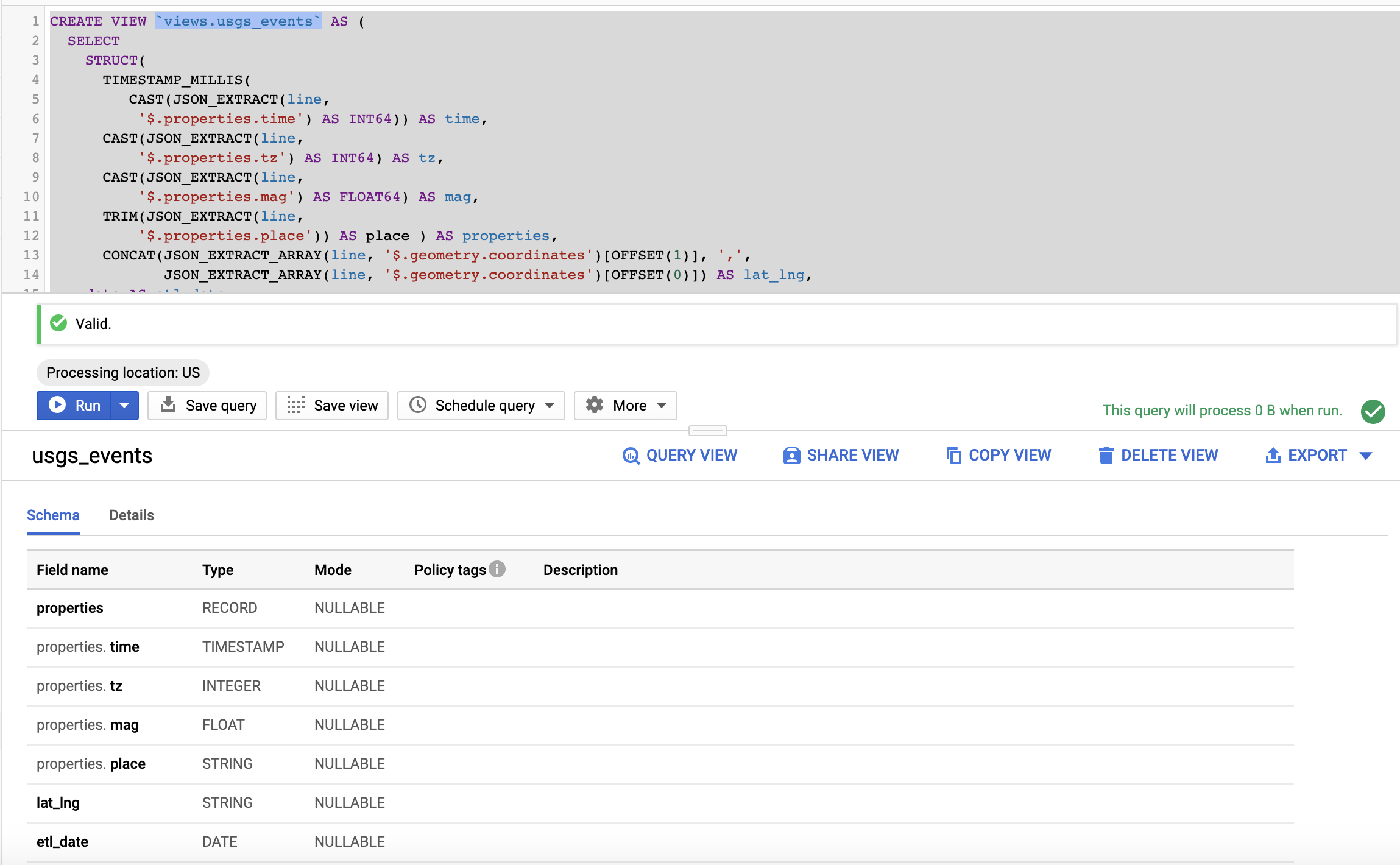
Note that latitude and longitude are concatenated as a comma-separated string for the next step.

Also note that I renamed date partition field to etl_date.
The view inherits the partition filter requirement so we can avoid any accident of scanning the entire dataset by accident:

SELECT * FROM `views.usgs_events`
WHERE etl_date BETWEEN DATE '2020-06-24' and DATE '2020-06-25'

Once the data is formatted, it is straightforward to visualize it on Google Data Studio:

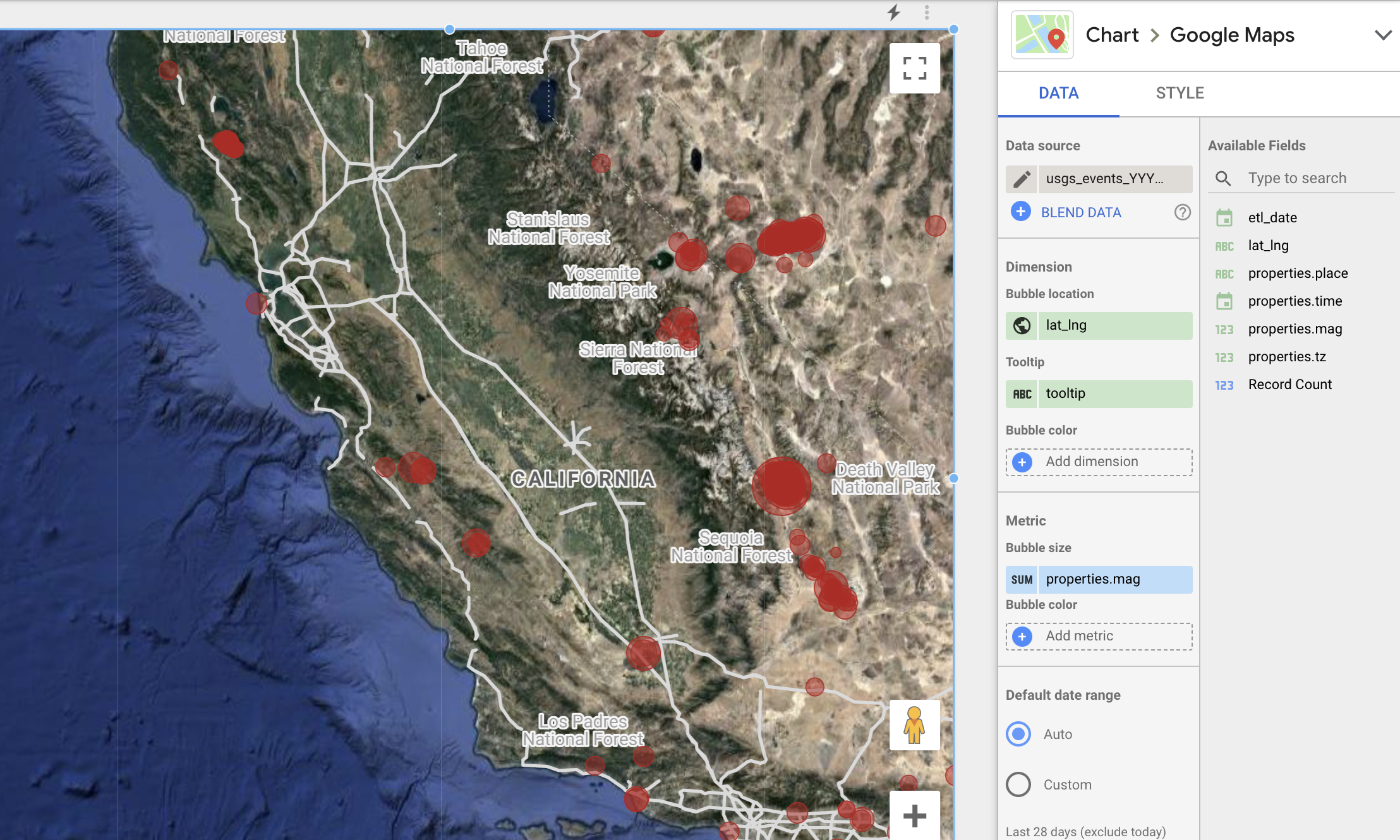
Here, Google Maps are selected as the chart type.
lag_lng is used for bubble location,
and property.mag is used as the bubble size.

ELT: Simple and powerful

In this post, I extracted the data simply with curl command without worrying about the file format or schema. The data was just dumped to Cloud Storage.
Then I created an externally partitioned table. Here again, I did not care to specify a schema.
At the very last step, I extracted the values from the raw strings and saved them as a structured view. I did so just by writing a SQL.
I could extract what I want with JSON_EXTRACT function for newline-separated JSON records. REGEXP_EXTRACT function would be useful for other types of file formats.

The parallelization of the query execution comes free, thanks to BigQuery.
Just imagine how slow the process would be if I had to

1. Specify the schema.
2. Write the transformation logic.
3. Configure the parallel processing for the transformation process by myself.

…before loading the data to the data warehouse.
What if the raw data’s schema suddenly changed?

I hope you are impressed by how quickly I processed and visualized the earthquake event data by choosing the simple and powerful ETL approach.
The computational benefit of transforming data in a massively-parallel data warehouse such as BigQuery would be even greater once I start extracting much more data continuously with a production-level extraction process such as this one.

A word of caution

I just demonstrated a case of efficiency gain with ELT.
However, ETL or ETLT can be more appropriate in other scenarios.
For example, masking or obfuscating personal identifiable data is very important before storing them in a data lake including Cloud Storage because it is much more costly to delete or modify a single record in a file partition after it’s loaded. (Think of a GDPR case a user requests a complete data erase.)

Extra: Animate the earthquake events on the map

Above visualization was created with this source code

I hope this introduction was informative and relatable to your business. If you would like to find out more what Anelen can do for your data challenge, please contact hello@anelen.co (.co, not .com don’t get your email lost elsewhere!) or schedule a free discovery meeting with the scheduler.

Daigo Tanaka, CEO and Data Scientist @ ANELEN